Table Of Content
Advanced data manipulation, integration of AI features, and proficiency with dynamic arrays stand out. Acquiring these skills equips you to handle complex datasets more efficiently, making it easier to derive meaningful insights and stay competitive in a data-driven landscape. This will depend on the type of data you have and the number of different parameters you will be tracking simultaneously. This is all you need to know about creating a graph in Excel. When it comes to Data Cleansing, find and replace is a great tool. Data cleaning is the most crucial step to eliminate incomplete and inconsistent data.
Industry-Specific Excel Charts
Then, under "Border Color," choose "Solid Fill." Under "Fill Color," choose the same color as the line in the chart. Change your transparency to the same transparency as the border color's transparency. In the menu that appears, choose the first type under the "Area" category. This falls under the previous bullet point, but I wanted to include it as its own point because it's one of the most overused data visualization effects. Maybe you pull data to convince your boss to adopt inbound marketing, give you an extra sliver of budget, or adjust your team's strategy -- among other things. Regardless of what you use data for, you need it to be convincing -- and if you display data poorly, the meaning of your data is more likely to get lost.
How to Automate Excel Monthly Report Creation to Save Time and Stop Errors
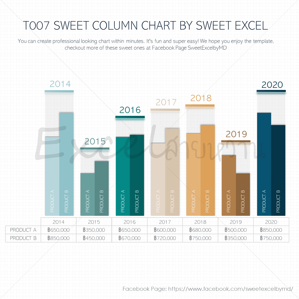
A chart, also known as graph, is a graphical representation of numeric data where the data is represented by symbols such as bars, columns, lines, slices, and so on. It is common to make graphs in Excel to better understand large amounts of data or relationship between different data subsets. Proper labeling and titling of the graph are essential for clarity and comprehension. Failing to label the axes, provide a clear title, and add a legend can confuse the audience and diminish the impact of the graph. Be sure to include all necessary labels and titles to ensure the graph is easily understood.
More Pro Chart Tips
Of course, this article has only scratched the surface of Excel chart customization and formatting, and there is much more to it. In the next tutorial, we are going to make a chart based on data from several worksheets. And in the meanwhile, I encourage you to review the links at the end of this article to learn more. To edit a data series, click the Edit Series button to the right of the data series. The Edit Series button appears as soon as you hover the mouse on a certain data series. This will also highlight the corresponding series on the chart, so that you could clearly see exactly what element you will be editing.
1 Final Thoughts and Takeaways for Choosing an Excel Chart Template Site
Next, double-click the shaded area on the chart (in this case, the red area) and a "Format Data Series" menu will appear. Click on "Fill" from the lefthand side, and choose "Solid Fill." Under "Fill Color," choose the same color as the line in the chart. You can change the transparency to whatever you'd like -- a transparency of 66% looks good. A line of a different color (in this case, red) will appear on top of our original line on the chart.
How to add a single vertical bar to a Microsoft Excel line chart - TechRepublic
How to add a single vertical bar to a Microsoft Excel line chart.
Posted: Fri, 27 May 2022 07:00:00 GMT [source]
Tutorials
Therefore, it's essential to consider the nature of the data and the message being conveyed when selecting a graph type in Excel. Graphs are a visual representation of data that can help users quickly and easily understand complex information. In Excel, graphs are used to present data in a visually appealing way, making it easier for users to analyze and interpret the data. You can click the Recommended Charts tab or the All Charts tab and start clicking your way down the list of chart types. Once the chart is selected, the ribbon above will show a Chart Design tab. You can go click on that or simply right-click your selected chart to save time.
It can become cluttered and hard to read, making it difficult to track progress effectively. 6) Indeed, a wide range of background colours may be chosen for the chart area and the dashed grid lines. Look at the chart given below to see the Gantt chart we have created.
For most Excel charts, such as bar charts or column charts, no special data arrangement is required. You’ll be able to create charts and graphs that quickly, cleanly, and clearly visualize your data for presentation. Clustered column charts display data changes over a period of time to make clear visualizations of rank among data sets. A line graph is a simple but highly effective way to see trends over time at a glance — even without the frills of bars, columns, or extra shading. Perfecting a chart in PowerPoint involves more than just adding data to a template.
Once your data is highlighted in the Workbook, click the Insert tab on the top banner. About halfway across the toolbar is a section with several chart options. Excel provides Recommended Charts based on popularity, but you can click any of the dropdown menus to select a different template.
A simple chart in Excel can say more than a sheet full of numbers. Find the series that seems to be invisible, select it and adjust formatting. If you have multiple series, you have the option of rearranging them on the chart. This will display the Edit Series window where you will need to specify the Series name and the Series values, in our case – the Budget column header and Budget values. Alternatively, right-mouse click on the axis labels and select Font. Right-click on the chart element and specify the colors you prefer from the fly-out menu.
How to Create a Scatter Plot in Excel - Lifewire
How to Create a Scatter Plot in Excel.
Posted: Thu, 09 Feb 2023 08:00:00 GMT [source]
Whether you’re a student, business professional, or just someone who loves organizing data, mastering the art of graph-making in Excel will elevate your data presentation game. In this article, we’ll walk you through the simple steps to create eye-catching graphs that will make your data pop and keep your audience engaged. Pie graphs usually compare parts of a whole, while bar graphs can compare pretty much anything ...
A new chart can also be inserted without having to highlight your data beforehand. To insert a chart, highlight the entire table including the headers. Given a set of data shown below, there are several ways to insert a new chart.
First, double-check your data selection to ensure it’s accurate. If the problem persists, you may need to adjust the graph’s axis scale or try a different graph type that better suits your data. Customizing your graph includes adding titles, labels, changing colors, adjusting scales, and more. This step is where you can get creative and make sure the graph reflects the story you want your data to tell.


No comments:
Post a Comment